Magnetic field visualization. II. Meridional slices

In part I of the magnetic field visualization we have introduced the basic nomenclature of the magnetic field and it's spectral components. And we have setup our environment to visualize the magnetic field and its components using Limace.jl.

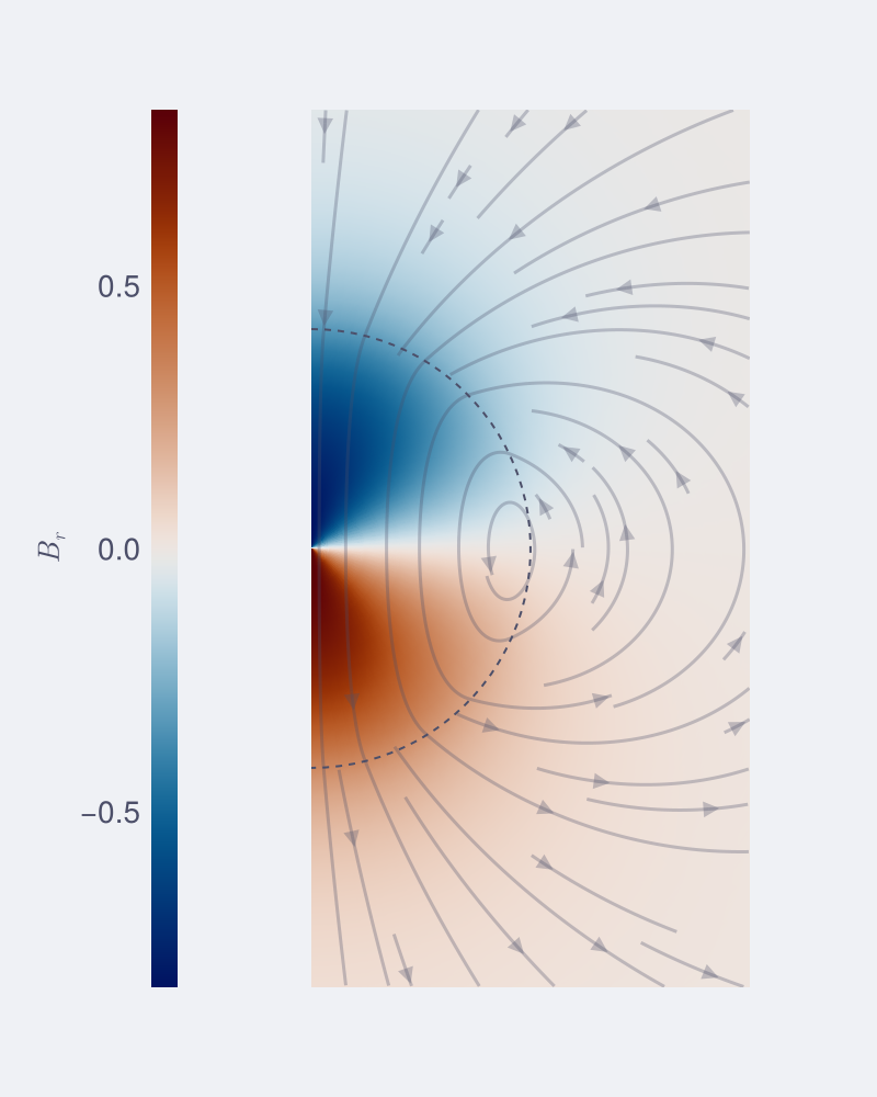
From here, we can visualize the actual magnetic field in two-dimensional plots, for example in meridional slices.

Let us define a BasisElement, consisting of one component of a Poloidal or Toroidal magnetic field element, of spherical harmonic degree $l$, order $m$ and radial degree $n$:

using Limace

N = 5
b = Insulating(N)

l,m,n = 1,0,1 # spherical harmonic degree l and order m , and radial degree n.
factor = 1.0 # amplitude or factor of the component

B_p_101 = BasisElement(b, Poloidal, (l,m,n), factor)

We have used here the basis Insulating, as defined in Gerick and Livermore (2024). At the surface (r=1), these basis elements match a potential field ($\sim -\nabla \Phi \sim -\nabla r^{-(l+1)}Y_l^m$). We can discretize this basis element B_p_101 on a grid

nr,nθ = 50,50
rmax = 2.0  #we can discretize at r>1 for this poloidal field.
r = range(1e-9,2rmax,length=nr)
θ = range(0,π,length=nθ)
x = r .* sin.(θ')
y = r .* cos.(θ')

ϕ = 0.0
B_disc = [discretize(B_p_101, r, θ, ϕ) for r in r, θ in θ] #discretize 3D magnetic field at each r, θ, ϕ
Br = real.(getindex.(B_disc,1)) #get only the radial component and take real part only of the complex field.

We can plot this meridional slice, extending to 0 ≤ x ≤ 2, -2 ≤ y ≤ 2.

#import and set theme
using CairoMakie
using CatppuccinMakieThemes #github.com/fgerick/CatppuccinMakieThemes.jl
_theme = CatppuccinMakieThemes.theme(CatppuccinMakieThemes.latte) #or CatpuccinMakieThemes.mocha for the dark mode.
CairoMakie.set_theme!(_theme)
div_colormap = :vik


f = Figure(size=(400,500))
ax = Axis(f[1,2], aspect=DataAspect())
xlims!(ax,0,rmax)
ylims!(ax,-rmax,rmax)
hidespines!(ax)
hidedecorations!(ax)
clim = maximum(abs,Br) #get color limits
s = surface!(ax, x, y, Br, colormap=div_colormap, colorrange=(-clim,clim), shading=NoShading)
Colorbar(f[1,1],s, vertical=true, label=L"B_r", flipaxis=false, height=400)

lines!(ax, sin.(θ), cos.(θ), color=_theme.textcolor, linestyle=:dash, linewidth=1) #plot r=1 half circle
f

Adding streamlines

In some cases it is useful and intuitive to illustrate the magnetic field lines. This is true, when a 2D description of the magnetic field is possible and therefore can be described by a stream function. For example, when the magnetic field is axisymmetric the field lines are two-dimensional at each meridional slice.

We can define some help functions to convert spherical vectors to Cartesian (needed for streamline plots).

function cart2sph(R)
	x,y,z = R
	r = sqrt(x^2+y^2+z^2)
	θ = atan(sqrt(x^2+y^2),z)
	ϕ = atan(y,x)
	return (r,θ,ϕ)
end

function sph2cartvec(u,R)
	r,θ,ϕ = R
	ur,uθ,uϕ = u
	ux = sin(θ)*cos(ϕ)*ur + cos(θ)*cos(ϕ)*uθ - sin(ϕ)*uϕ
	uy = sin(θ)*sin(ϕ)*ur + cos(θ)*sin(ϕ)*uθ + cos(ϕ)*uϕ 
	uz = cos(θ)*ur - sin(θ)*uθ
	return (ux,uy,uz)
end

function streamofb0(x,z, B0)
	R = cart2sph((x,0,z))
	b = real.(sph2cartvec(Limace.Discretization.discretize(B0,R...),R))
	return Point2(b[1],b[3])
end

And then simply add the streamlines to the previous plot axis ax:

streamplot!(ax,(x,z)->streamofb0(x,z,B_p_101),-rmax..rmax,-rmax..rmax; color=x->_theme.textcolor[], arrow_size=10,density=0.8, alpha=0.3, stepsize=0.01, maxsteps=1_000_000)
f

References

• Gerick, F. and Livermore, P. W. (2024). Interannual Magneto–Coriolis Modes and Their Sensitivity on the Magnetic Field within the Earth's Core. Proc. R. Soc. A 480, 20240184.

go back