Magnetic field visualization. I. Theory and setup

Geophysicists like to speak about Earth's magnetic field in terms of spherical harmonic degrees $l$ and orders $m$, in internal and external, toroidal and poloidal components. Sometimes, it is nice to come back to the actual shape of the magnetic field and to visualize it in space to get some intuition on what we are actually discussing.

Here, I will outline how to visualize components of the magnetic field $\mathbf{B}$ used to model waves internal to the Earth's core using the Limace.jl package.

For a reminder, I will start with the very technical description of the magnetic field for the unfamiliar reader. For a (much) more rigorous and detailed description of the theoretical aspects of the geomagnetic field, I refer to Backus et al. (1996).

Theoretical description of the magnetic field

The magnetic field $\mathbf{B}$ can be described by two scalar functions $P$ and $T$, known as the poloidal and toroidal scalars, so that

where $\mathbf{r}=r\mathbf{e}_r$ with the radius $r$ and the unit vector in the radial direction $\mathbf{e}_r$, for spherical coordinates $(r,\theta,\phi)$. This is a consequence of not allowing for magnetic monopoles ($\boldsymbol{\nabla}\boldsymbol{\cdot}\mathbf{B}=0$).

These scalars $P,T$ are commonly further separated into radial functions $P_n(r), T_n(r)$ and the spherical harmonics $Y_l^m(\theta,\phi)$, so that

where $\alpha_{lmn}$ and $\beta_{lmn}$ are scalar coefficients determining the amplitude of each component.

So far, we have not distinguished between regions that are electrically conducting or assumed insulating. For simplicity, let us assume that only the core of the Earth is conducting and everything above (mantle, crust, ionosphere and magnetosphere) is electrically insulating. Then, we can separate our description of the magnetic field into two regions, one interior and one exterior to the core. In the insulating exterior, $r>1$ (for the radius of the core fixed to $r=1$), the magnetic field must satisfy

i.e. no current. This condition translates to

Since $\boldsymbol{\nabla}\boldsymbol{\cdot}\mathbf{B}=0$, we require $\nabla^2 \Phi = 0$ so that $\Phi \sim l P_n(1)r^{-(l+1)}Y_l^m$. The required continuity of the magnetic field from the interior to the exterior is equivalent to boundary conditions at $r=1$:

In addition, the description in the interior down to $r=0$ requires that the radial functions require a regularity condition (Livermore et al., 2007), namely $P_n,T_n \sim r^l f(r^2)$. What remains to be defined are the radial functions $P_n,T_n$, subject to the boundary conditions (5).

Examples of functions based on Jacobi polynomials $J_n^{(a,b)}(x)$ can be found in Li et al. (2010) and Gerick and Livermore (2024). We shall focus here on the latter, as this is the basis implemented in Limace.jl.

Poloidal and toroidal scalars satisfying the insulating boundary conditions (5) are given by

with the normalization factors

The definition of a basis of poloidal and toroidal field vectors for a magnetic field in a full sphere, satisfying the insulating boundary condition at $r=1$ is hereby complete. We can now move on to the visualization of components of this magnetic field within the Limace.jl package.

Magnetic field components in Limace.jl

Let us now visualize some of these scalar functions using Limace.jl. First, we need to set up our working environment, if we don't have one already available.

import Pkg; Pkg.add(url="https://github.com/fgerick/Limace.jl.git")

Pkg.activate(".")

Pkg.add(["CairoMakie"; "WGLMakie"])

using Limace
using CairoMakie

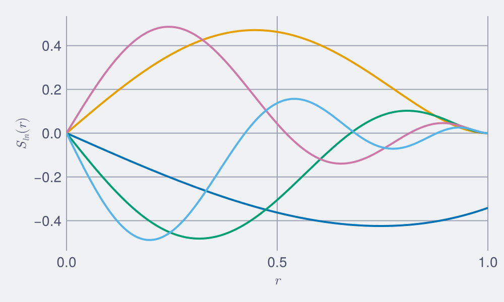
With the environment set up, we are ready to visualize some of the scalar functions defined in (6). For example, the first few degrees $S_{11}(r),...,S_{15}(r)$ are plotted as

using Limace
using CairoMakie

b = Insulating(5) #defines the basis
l,m = 1,0
S(l,n) = r->Limace.s(b, l,m,n,r) #access the poloidal scalar function (identical for all m)

f = Figure(size=(500,300))
ax = Axis(f[1,1], xlabel=L"r", ylabel=L"S_{ln}(r)")
xlims!(ax,0,1)
for n in 1:b.N
	lines!(ax,0..1,S(l,n), linewidth=2)
end
f

It is interesting to note here, that only the $n=1$ degree has a non-zero component at $r=1$. Therefore, only this single degree contributes to the magnetic field observable outside of the core. By definition, all $T_{ln}(1)=0$.

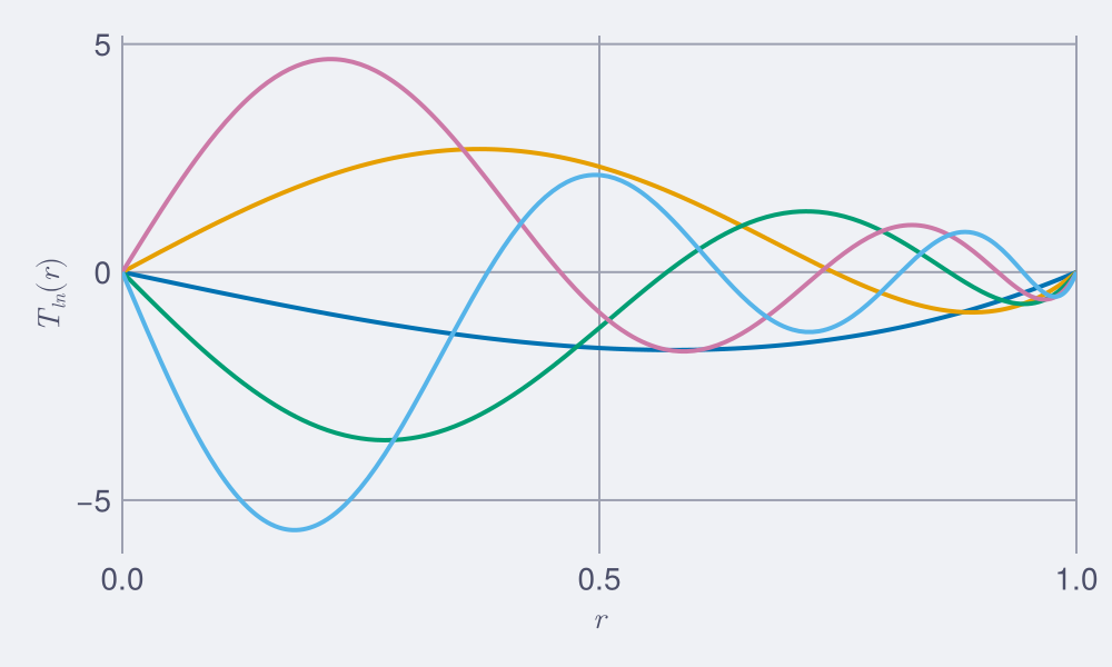
T(l,n) = r->Limace.t(b, l,m,n,r) #access the toroidal scalar function (identical for all m)

f = Figure(size=(500,300))
ax = Axis(f[1,1], xlabel=L"r", ylabel=L"T_{ln}(r)")
xlims!(ax,0,1)
for n in 1:b.N
	lines!(ax,0..1,T(l,n), linewidth=2)
end
f

Summary

We have recalled the definition of a magnetic field basis in terms of poloidal and toroidal components, including the definition of the scalar functions $P$ and $T$. One defintion of these scalar function, implemented in Limace.jl was outlined and we have setup our Julia environment to use Limace.jl and CairoMakie.jl to visualize a few degrees of the scalar functions. From here, we are in the position to visualize the actual magnetic field.

References

• Backus, G.; Parker, R. and Constable, C. (1996). Foundations of Geomagnetism (Cambridge University Press).

• Livermore, P. W.; Jones, C. A. and Worland, S. J. (2007). Spectral Radial Basis Functions for Full Sphere Computations. J. Comput. Phys. 227, 1209–1224.

• Gerick, F. and Livermore, P. W. (2024). Interannual Magneto–Coriolis Modes and Their Sensitivity on the Magnetic Field within the Earth's Core. Proc. R. Soc. A 480, 20240184.

• Li, K.; Livermore, P. W. and Jackson, A. (2010). An Optimal Galerkin Scheme to Solve the Kinematic Dynamo Eigenvalue Problem in a Full Sphere. J. Comput. Phys. 229, 8666–8683.

go back